Using Latent Distance as a Proxy for Uncertainty

Neural networks are confident about everything. Ask one to predict something it's never seen before and it'll give you an answer with the same conviction as something it trained on a million times. That's a problem. If you're using a model in the real world, you need to know when it's guessing.

This article walks through three ways to measure how uncertain a model is, starting with the standard expensive approaches and ending with a cheaper one that turned out to work better.

Code for everything here: github.com/ali77sina/distance-based-on-certainty

What does "uncertainty" mean here?

Imagine you train a model to predict a curve. You show it data points between -3 and +3, and it learns the shape of the curve in that region. Now you ask it to predict at x = 10. It'll give you a number, but it has no idea what the curve does out there. It's extrapolating blindly.

A good uncertainty method should say "I'm confident" inside the training region and "I'm guessing" outside of it.

The test

I trained models to learn sin(x) (just a wavy curve) using data between -pi and +pi. Then I tested them on the much wider range of -3pi to 3pi. Most of the test range is territory the model has never seen.

Method 1: Deep Ensemble (the expensive standard)

Train 10 separate models on the same data. Each one learns slightly different things because of random initialization. At prediction time, run all 10 and see how much they disagree. If they all say roughly the same thing, the prediction is probably right. If they're all over the place, the model is uncertain.

The catch: you need to train and store 10 separate models, and run all of them at inference time. That's 10x the compute.

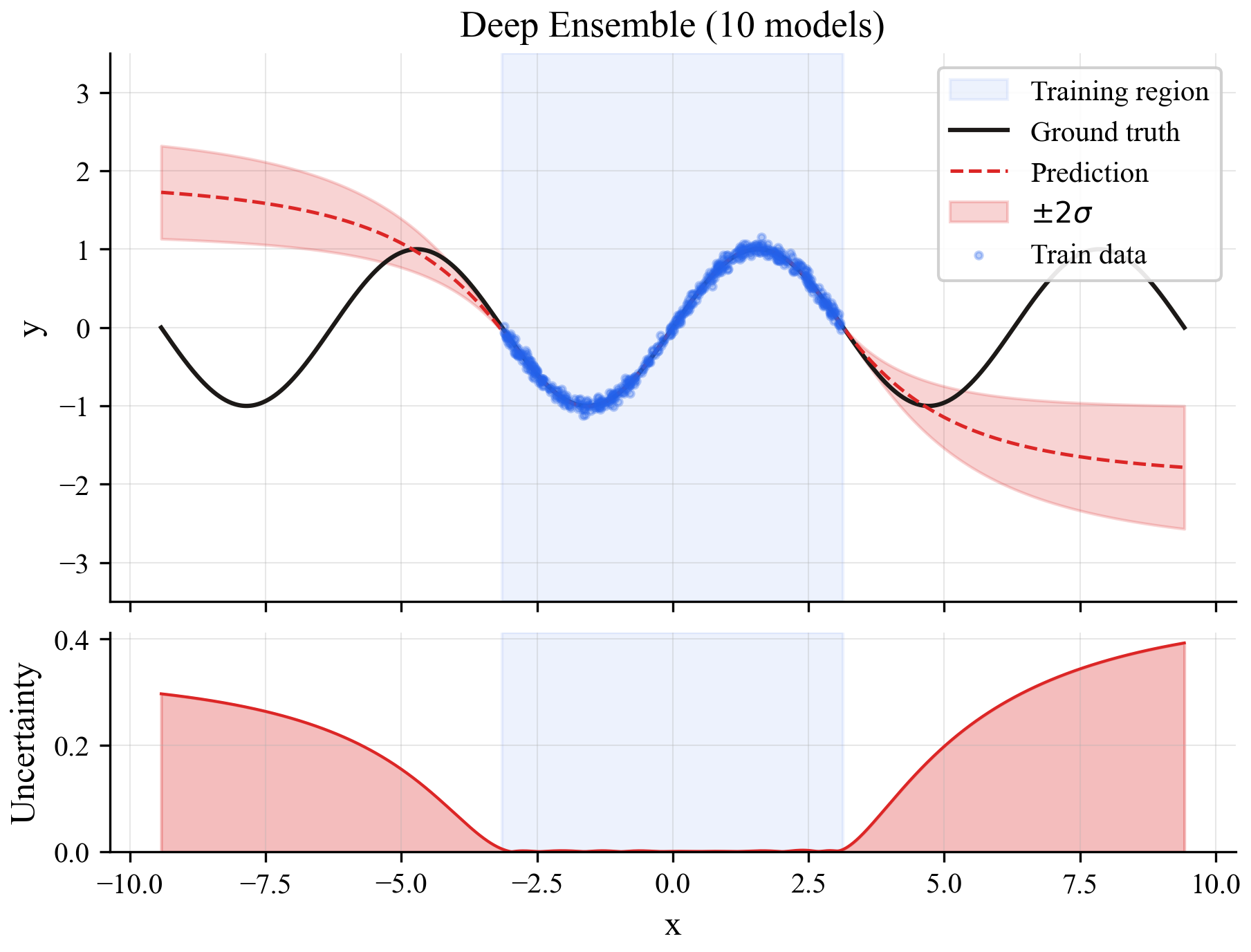
The top plot shows predictions (blue line) with uncertainty bands (shaded region). The bottom shows the raw uncertainty signal. Inside the training region (blue background), uncertainty is low. Outside, it rises gradually.

Method 2: Bayesian Neural Network

Instead of training 10 separate models, train one model where each weight is a probability distribution instead of a fixed number. At prediction time, sample from those distributions 10 times and see how much the predictions vary.

Conceptually similar to the ensemble but uses one model instead of ten. Still needs multiple forward passes at inference.

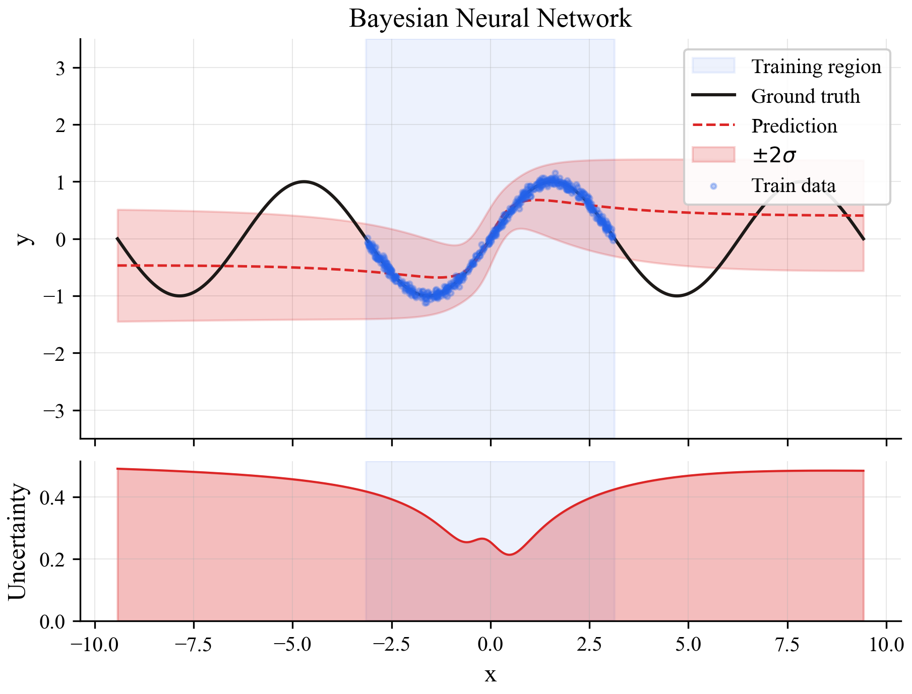
The result is similar to the ensemble but noisier. The uncertainty signal is there but less clean, which is typical for this approach with only 10 samples.

Method 3: Latent distance (the cheap one)

This is the idea I wanted to test. Every neural network has an internal representation of its input, a compressed version that lives in a hidden layer somewhere in the middle of the network. During training, the model builds up a mental map of what "normal" inputs look like in this internal space.

The idea: at inference time, check if the new input's internal representation looks like anything the model saw during training. If it's close to known territory, trust the prediction. If it's in uncharted space, don't.

This only needs one model and one forward pass. No ensembles, no sampling.

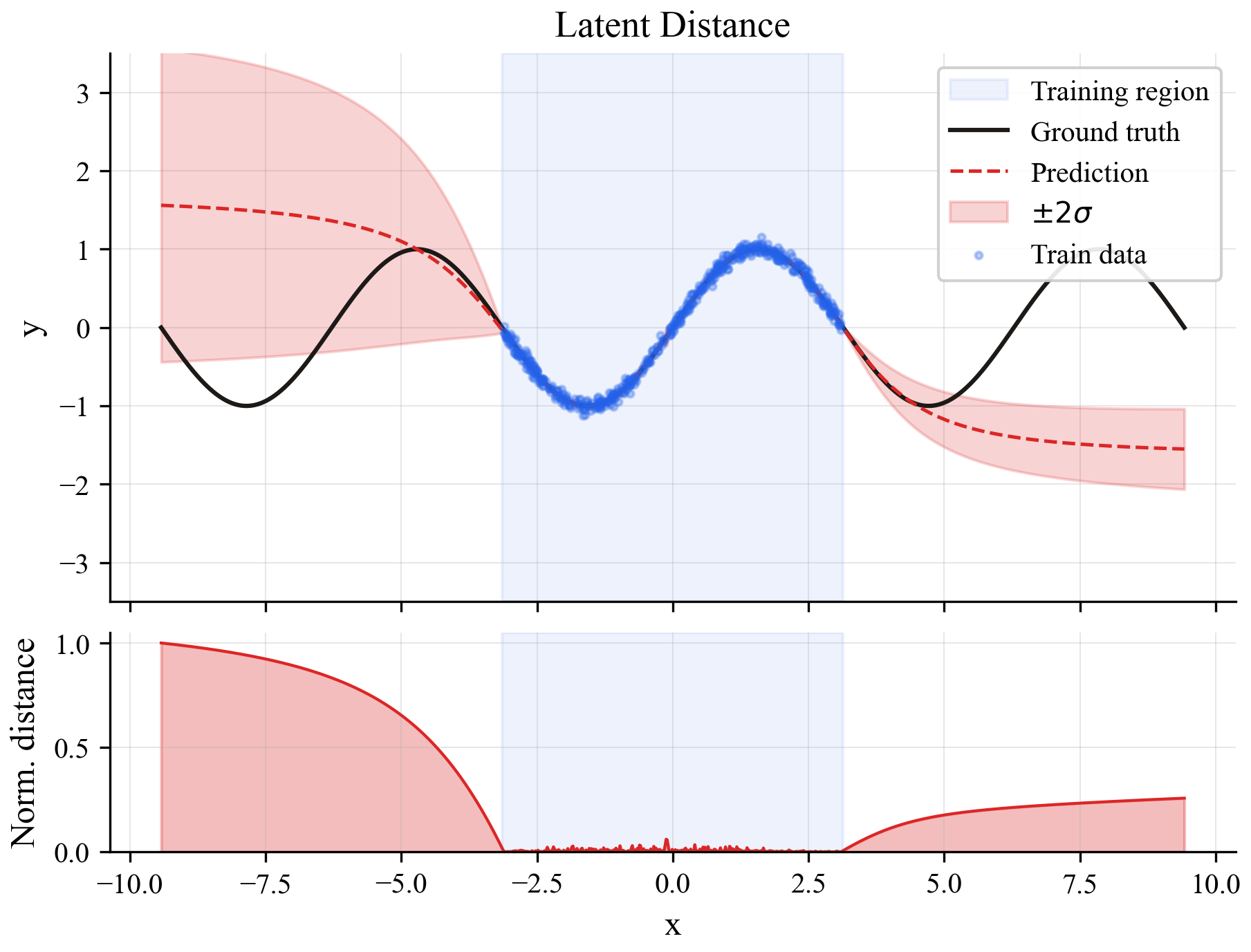
The uncertainty signal is the sharpest of the three. Near-zero inside the training region, then it jumps at the boundaries. It's basically a binary signal: "I've seen this" or "I haven't."

Side-by-side comparison

Here's all three methods on the same plot:

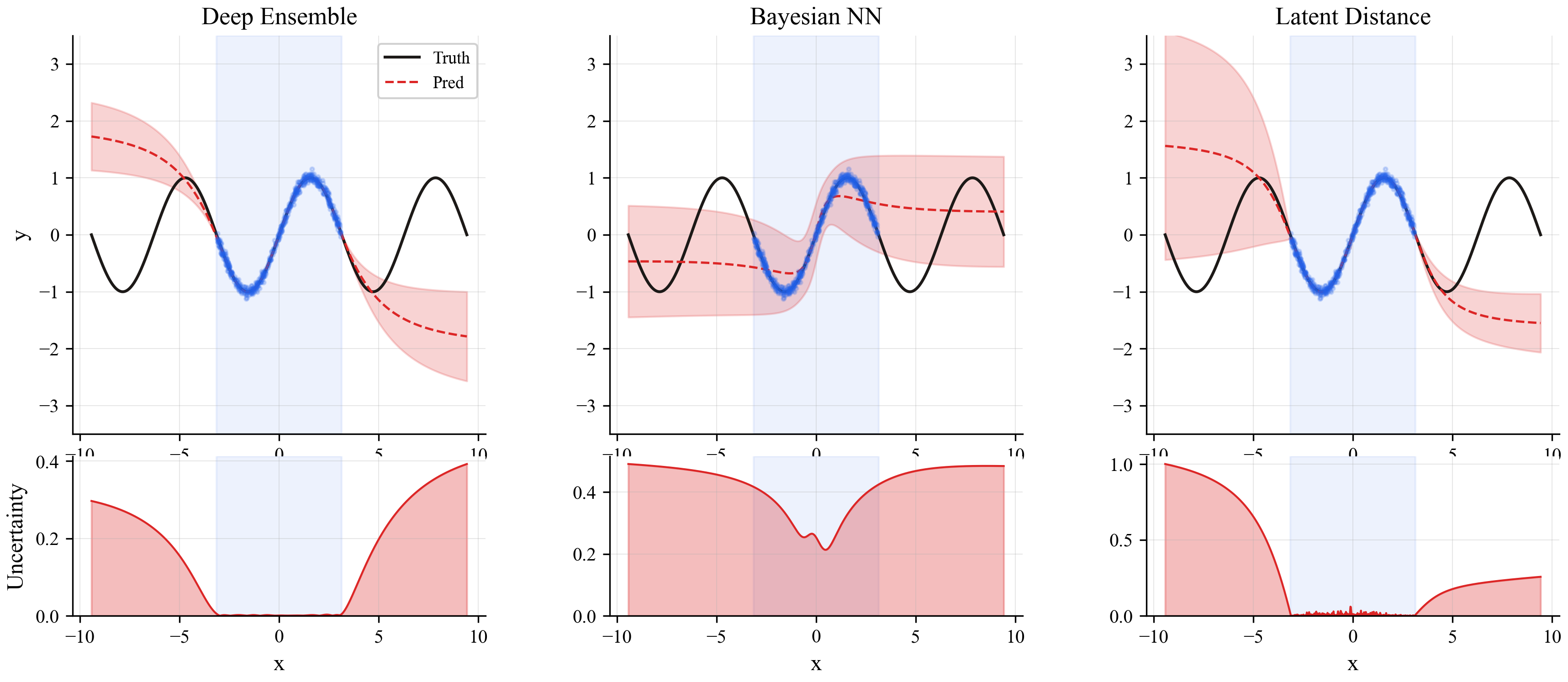
The ensemble (left) gives a smooth, gradual rise. The Bayesian NN (middle) is similar but noisier. The latent distance method (right) has the crispest boundary between "known" and "unknown" territory.

Looking inside the model's brain

What does the model's internal representation actually look like? Here's a visualization of the latent space after compressing it to 2 dimensions with PCA:

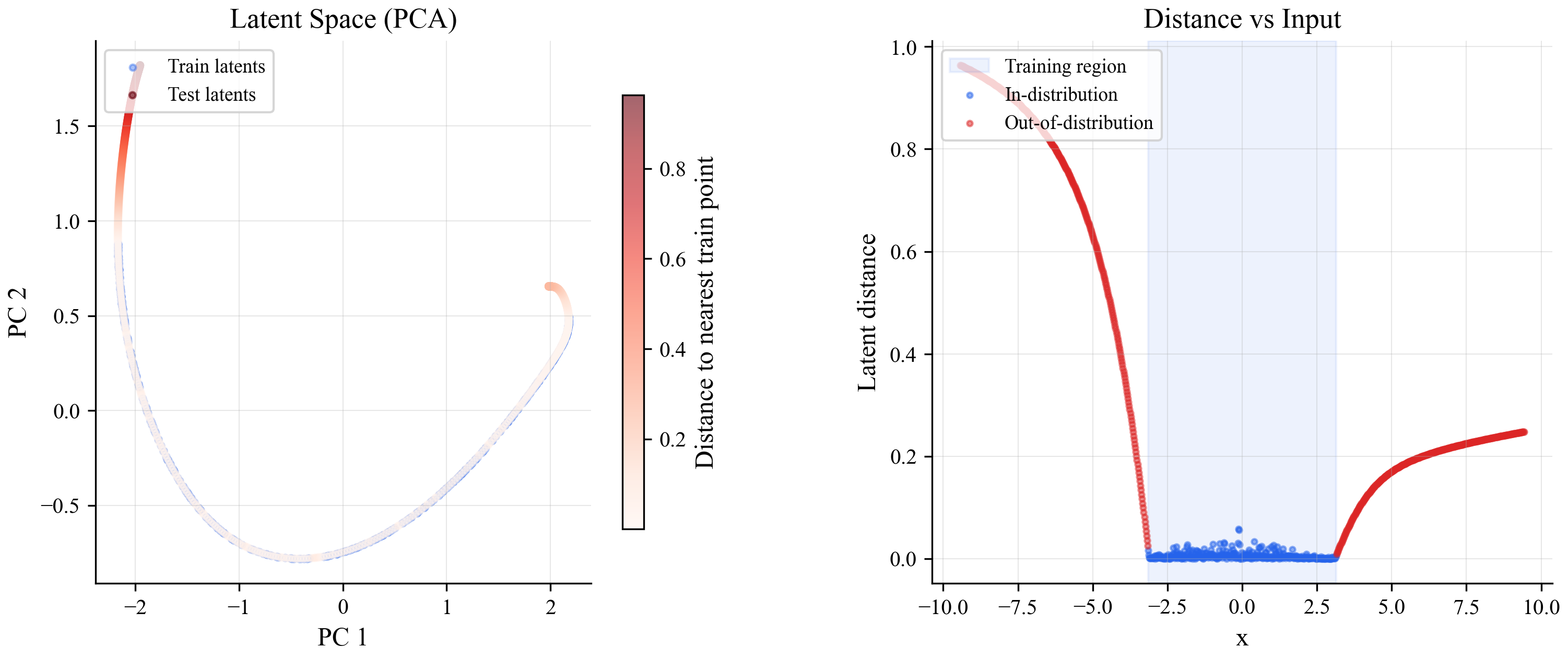
On the left, blue dots are training points and red dots are test points. The training points form a tight curve. Points from outside the training region scatter away from it. On the right, you can see how distance from training data maps directly onto the input: low inside the training range, high outside.

The cost comparison

All three methods detect uncertainty on this problem. But they don't cost the same:

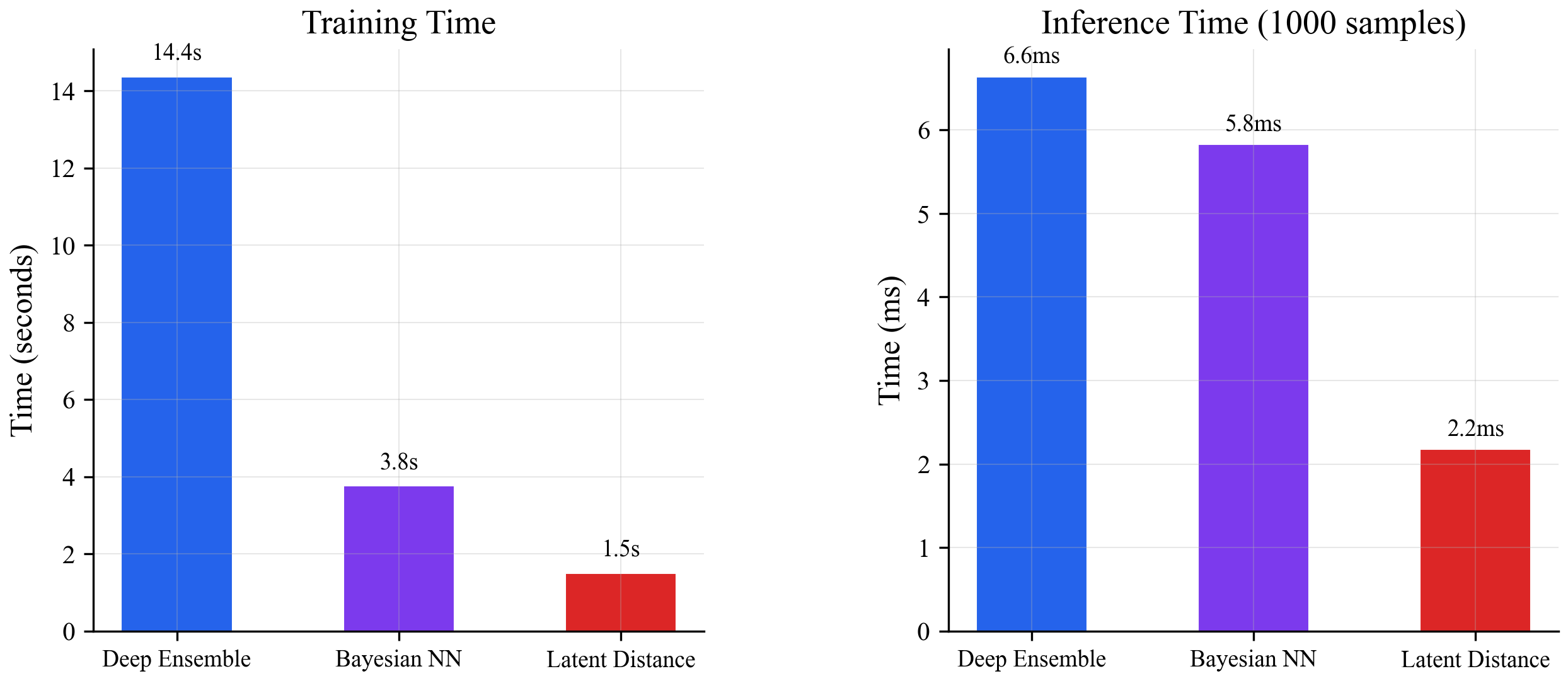
The ensemble needs 10 models trained separately (14.4s total training, multiple forward passes at inference). The Bayesian NN needs special training with weight distributions (3.8s, still needs 10 forward passes). The latent distance method needs one normal model (1.5s) and a single forward pass plus a quick lookup.

Does it scale?

As you add more ensemble members or more Bayesian samples, both of those methods get more accurate but also more expensive. The latent distance method's cost is flat:

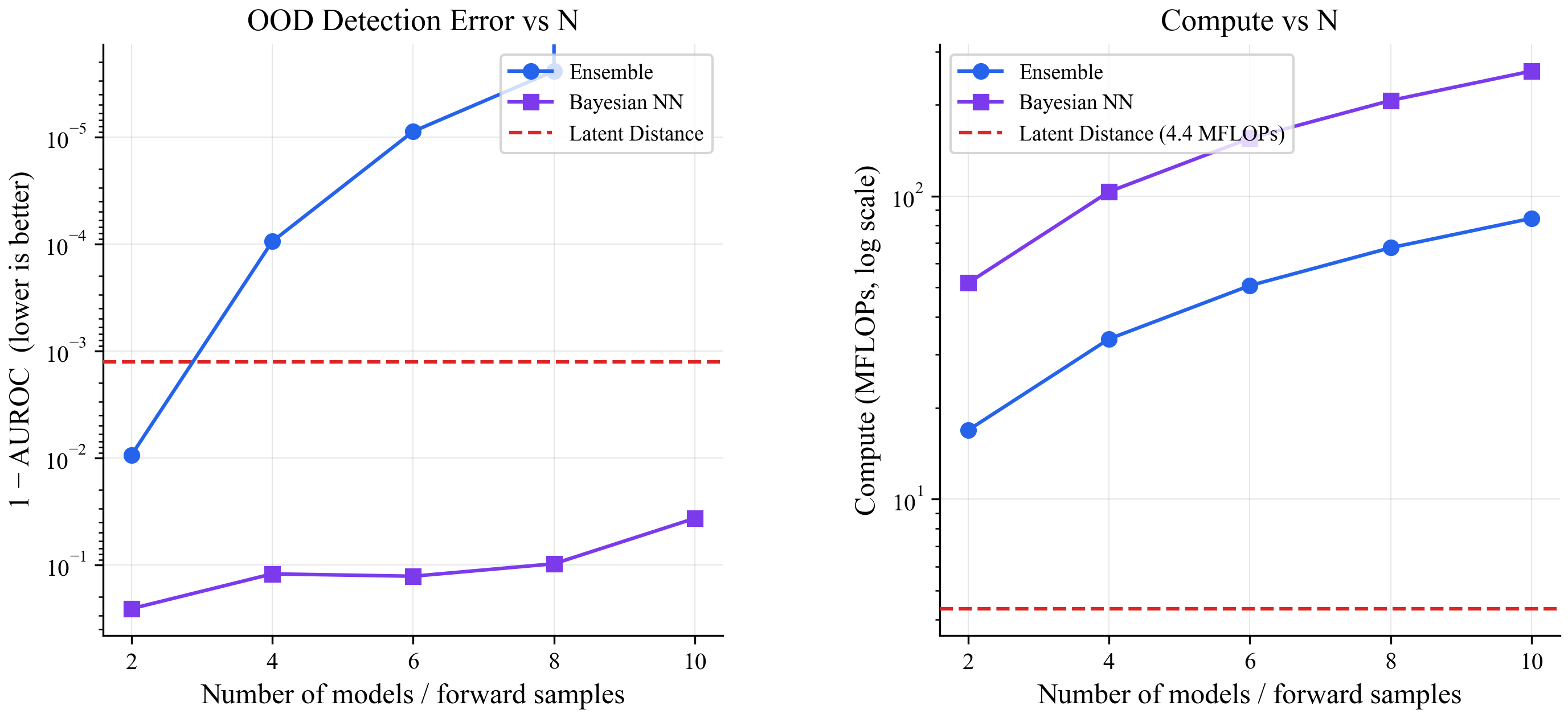
Left: all methods detect out-of-distribution points nearly perfectly on this toy problem (AUROC close to 1.0). Right: the ensemble and Bayesian NN cost scales linearly with the number of models/samples. The latent distance method stays at the same cost regardless.

The hard test: real images

Sin(x) is too easy. Everything works on toy problems. So I tested on something harder: train a classifier on handwritten digits (MNIST), then see if the uncertainty method can tell when it's shown fashion items (FashionMNIST) instead of digits.

The naive version of latent distance (PCA + nearest-neighbor search) collapsed completely: 0.46 AUROC, which is worse than flipping a coin. Compressing the internal representation down to 2 dimensions with PCA threw away too much information. The ensemble (0.979) and Bayesian NN (0.957) handled it fine.

The first histogram shows the problem. The uncertainty scores for real digits (blue) and fashion items (orange) completely overlap. The method can't tell them apart.

Fixing it with better density estimation

The internal representation itself wasn't the problem. It was the crude way I was measuring "distance" in it. PCA + nearest-neighbor is like trying to understand a city by looking at a 2D map when you need the full 3D model.

I tried two fixes, both using the full internal representation without compressing it:

Gaussian Mixture Model (GMM): after training, fit a statistical model (a mixture of bell curves in high-dimensional space) to the training data's internal representations. At inference, ask "how likely is this new point under that statistical model?" Low likelihood means the model hasn't seen anything like it.

Normalizing Flow: a small neural network that learns to transform the training data's internal representations into a simple standard distribution. Trained alongside the main model. At inference, points that don't transform cleanly are flagged as unfamiliar.

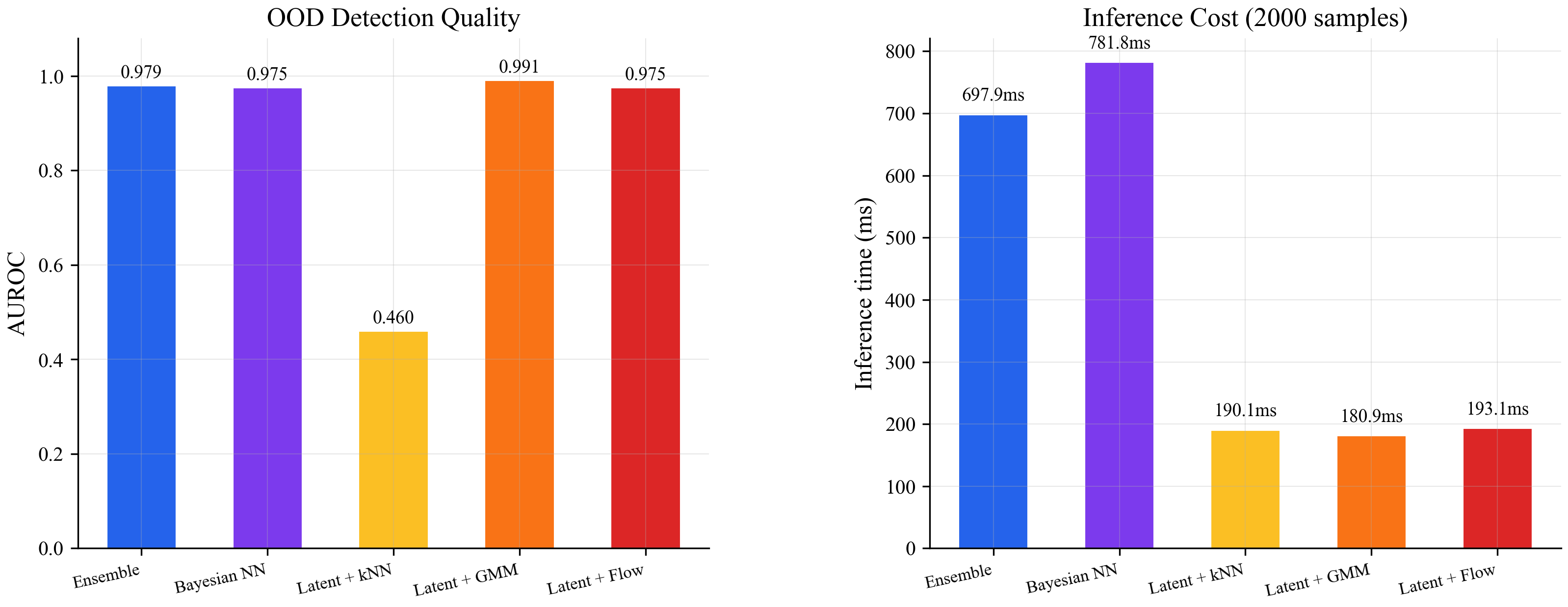
The GMM hit 0.991 AUROC, beating the ensemble (0.979). The flow matched the ensemble at 0.975. Both ran inference in about 190ms for 2000 samples. The ensemble took 698ms and the Bayesian NN took 782ms. Better accuracy at roughly 4x lower cost.

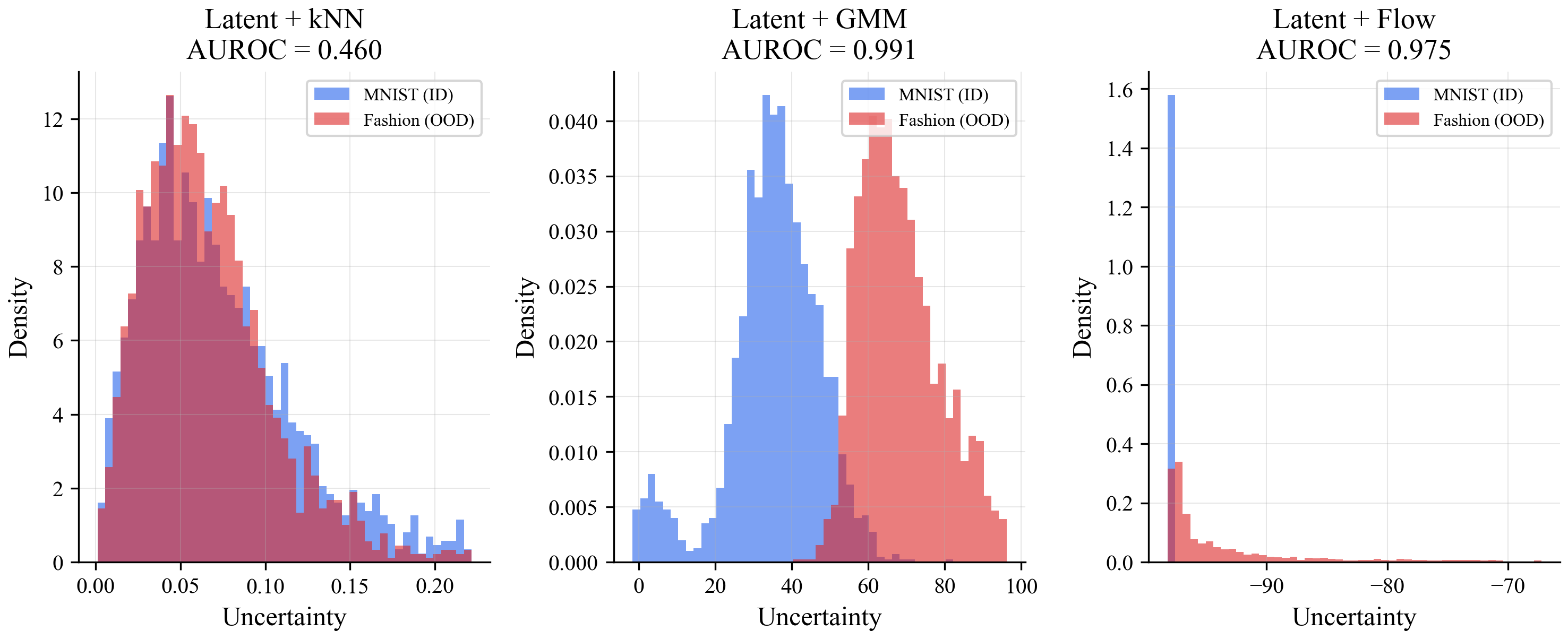
Now look at the histograms. The kNN version (top-left) is still a mess. But the GMM (bottom-left) cleanly separates digits from fashion items. The flow (bottom-right) does the same.

What this all means

The model's internal representation already contains the information needed to know when it's in unfamiliar territory. The expensive methods (ensembles, Bayesian NNs) work by training multiple models and seeing if they disagree. But you can skip all that and just ask: "does this input look like something I've seen before, based on what's happening inside my own network?"

The practical recipe is simple:

1. Train your model normally, with a bottleneck layer somewhere in the middle
2. After training, fit a GMM on the internal representations of your training data
3. At inference, one forward pass through the model, then score the internal state against the GMM

One model, one forward pass, better results than running 10 models in parallel.